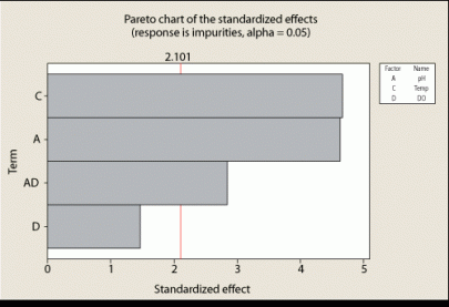
Because these parameters and interactions are not significant, they may be treated as random noise and the model for this attribute is reduced as shown in Figure 5. A mathematical model was generated using the significant factors (pH and temperature) from Figure 3 and the significant interaction (pH and dissolved oxygen [DO]):
Impurities = Constant + α(pH) + β(temperature) + γ(DO) + δ(pH) (DO)
where: Constant is the intercept generated by the DOE analysis
α, β, γ, and δ are the coefficients generated by the DOE analysis for each parameter or interaction.
Positively signed coefficients indicate the CQA increases with an increase of the parameter; negatively signed coefficients indicate the CQA decreases with an increase of the parameter. The model equation is a regression, or best fit, from the data for the experiment, and therefore, is valid for the specific scale conditions of the experiment including the ranges of the parameters tested. Models are tested for their “goodness of fit” or how well the model represents the data. The simplest of these tests is the coefficient of determination, or R-squared. Low R-squared values (such as below 50%) indicate models with low predictive capability, that is, the parameters evaluated across the defined range do not explain the variation seen in the data.
This model only represents what would be expected on average for this CQA from the unit operation(s) tested in the study. Even so, the model is a fit to the most likely mean. Recognizing that any model has uncertainty, the model can also be represented with a confidence interval (e.g., 95%) around that mean. Individual runs will also show day-to-day variation around that mean. A single-run value for the attribute cannot be predicted, but a range in which that value will likely fall can be predicted. This range for the single-run value is called the prediction interval (e.g., 95%) for the model. Empirical models such as these are only as good as the data and conditions from which they are generated and are mere approximations of the real world.
Despite the limitation, these empirical models relate not only what parameters have a statistical impact on a CQA, but also the relative amount of that impact. The range through which the parameter is tested in the study has an important relationship to the model generated. For example, perhaps the parameter temperature was initially assigned as high risk. If temperature is only tested through a tight range, the parameter may have little to no impact to CQAs in the study; its effect may be no greater than the inherent variability. If temperature is not statistically significant for the range studied (i.e., its PAR), it is designated as a non-CPP, but only for that PAR. If the temperature should ever move outside the studied PAR, there is a potential risk that it could have a quality impact become critical.
Some organization quality groups rely on the original risk assessment of the process parameter. If this parameter’s severity was initially rated high, this parameter can remain designated as critical but should be designated as a low-risk CPP as long as the parameter is in its PAR. Parameters outside the PAR would be considered outside the allowable limits for that process step because there has been no study of the parameter outside of this range.
If curvature is detected during earlier DOE stages, or if the optimization of any CQA or process performance attribute is needed, then response-surface experimental designs are used. These designs allow for more complex model equations for a CQA (or performance attributes). Two of the simpler response-surface designs are the central composite and Box-Behnken. Both designs can supplement existing full-factorial data. The central-composite design also extends the range of parameter beyond the original limits of the factorial design. The Box-Behnken design is used when extending the limits is not feasible. The empirical models are refined from these studies by adding higher-order terms (e.g., quadratic, polynomial). Even if these higher-order terms are not significant, adding more levels within the parameter ranges will improve the linear model.
Because most empirical models are developed with small-scale experiments, the models must be verified on larger scale and potentially adjusted. Applying the knowledge of scale-dependent and scale-independent parameters while developing earlier DOE designs reduces risk when scaling-up to larger pilot-scale and finally full-scale processes. The models from small-scale studies predict which parameters present the highest impact (risk) to CQAs. Priority should be given in the study design to those high-risk parameters, especially if they are scale-dependent. Since the empirical models only predict the most likely average response for a CQA, several runs at different parameter settings (e.g., minimum, maximum, center point) are required to see if the small-scale model can still apply to the large-scale process.
Significance and criticality
Statistical significance is an important designation in assessing the impact of changes in parameters on CQA. It provides a mathematical threshold of where the effects vanish into the noise of process variability. Parameters that are not significant are screened out from further study and excluded from empirical models.
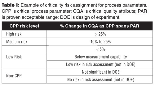
A CQA may be affected by critical parameters in several different unit operations (see the Cause-and-Effect Matrix in Part 1 of this article [5]). Characterization study plans may not be able to integrate different unit operations into the same DOE study. Consequently, several model equations may exist for a single CQA; each model is composed of parameters from different unit operation. The relative effect of each parameter on the CQA can be calculated from these models using the span of the PAR for each parameter. The relative impact of each parameter on the CQA is based on the range of its acceptance criteria. Sorting each parameter from highest to lowest, the criticality of each parameter can be assigned from high to low. Table I is an example of one method for assigning the continuum of criticality.
The steps in determining the continuum of criticality for process parameters are summarized as follows:
• Show statistically significance by DOE
• Relate significant parameters to CQAs with empirical model
• Calculate impact of all parameter from model(s) for CQA
• Compare the parameter’s impact on the CQA to the CQA’s measurement capability
• Assign parameter risk level based on impact to CQA
• Update initial risk assessment for parameters.

As process validation Stage 2 (process qualification) begins, criticality is applied to develop acceptance criteria for equipment qualification and process performance qualification. Finally, in process validation Stage 3 (continued process verification), criticality determines what parameters and attributes are monitored and trended.
In the third and final part of this article, the author applies the continuum of criticality for parameters and attributes to develop the process control strategy and study its influence on the process qualification and continued process verification stages of process validation.
References
1. FDA, Guidance for Industry, Process Validation: General Principles and Practices, Revision 1 (Rockville, MD, January 2011).
2. ICH, Q8(R2) Harmonized Tripartite Guideline, Pharmaceutical Development, Step 4 version (August 2009).
3. ICH, Q9 Harmonized Tripartite Guideline, Quality Risk Management (June 2006).
4. ICH, Q10, Harmonized Tripartite Guideline, Pharmaceutical Quality System (April 2009).
5. M. Mitchell, BioPharm International 26 (12) 38-47 (2013).
Mark Mitchell is principal engineer at Pharmatech Associates.